

Because it can accurately anticipate output growth, inflation, and interest rates – three crucial factors for the overall economy and financial assets – the bond market is sometimes referred to as the “smart money” on Wall Street by traders. Based on this belief, investors sometimes pay close attention to bonds and the peaks and valleys of the yield curve to learn more about future economic performance and developing trends. Given how interconnected the financial system is, signals from one market might sometimes serve as an indication, even a leading one, and a forecasting tool for another that is slower or less effective at integrating new data.
This article will examine the Treasury market to see how the yield curve’s shape and slope might provide hints about anticipated future equity returns and sector leadership by revealing information about the economic cycle. Before starting, it is vital to familiarise yourself with critical ideas.
CURVE FOR TREASURY YIELD
The Treasury yield curve is a graphical depiction that shows the interest rates on government bonds for all maturities, from overnight to 30 years, across several tenors. It illustrates an investor’s return by lending money to the U.S. government for a certain time. The asset yield is shown on the graph’s vertical axis, and the borrowing term is shown on the graph’s horizontal axis.
Longer-term debt instruments often provide better yields than short-dated ones to offset additional risks like inflation and length. Therefore the curve may assume various forms in healthy settings (see figure below). For instance, the yield on a 30-year government bond is often more significant than that of a 10-year note, which should be higher than that of a 2-year Treasury note.
The U.S. Yield Curve
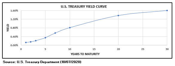
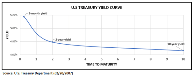
Even though it’s uncommon, there are situations when long-term security may provide a lower return than a short-term investment, resulting in a term structure of interest rates that slopes downward. When this happens, the yield curve is said to have inverted.
The yield curve often inverts when the central bank raises short-term rates to avoid overheating to the point where it restricts activity and clouds the outlook for the economy. Investors wager that interest rates will need to decrease in the future to handle a potential downturn and disinflation when monetary policy becomes too restrictive. These presumptions lead to a decline in longer-dated bond rates and an increase in short-term bond rates, which inverts the Treasury curve.
Inversions have historically often predicted approaching recessions. An economic downturn has followed each 3-month to 10-year or 3m10y yield curve inversion since the end of World War II.
U.S. Yield Curve inverted
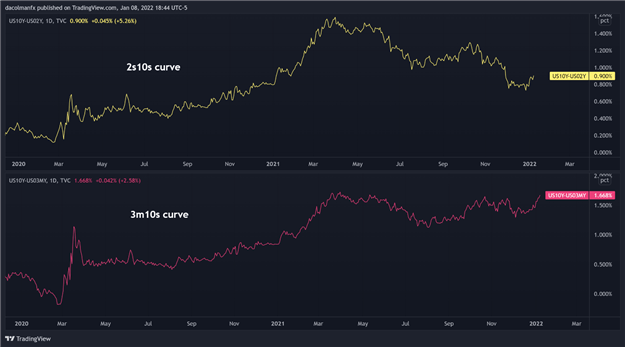
Traders often compare two rates at two different maturities and refer to their spread, defined in basis points, as “the yield curve” instead of concentrating on the Treasury market’s overall interest rate term structure. The following curves are the ones that are most commonly discussed and examined in financial media:
- The 2-year/10-year curve sometimes referred to as the twos-tens or 2y10y: is the spread between the yield on 10-year Treasury bonds and the yield on 2-year Treasury notes.
- The 3-month/10-year curve sometimes referred to as the 3m10y or three-month-tens curve: The yield differential between the 10-year Treasury bond and the 3-month Treasury bill is shown by this curve.
CURVES FOR 2S10S AND 3M10S SINCE 2020
Modifications to the yield curve
The difference between long-term and short-term Treasury rates will fluctuate with changes in economic activity, inflation expectations, monetary policy outlook, and liquidity circumstances. The curve is considered to steepen when the spread widens, and the gap between long- and short-dated rates grows. On the other hand, the yield curve is considered to flatten when the term spreads contract.
The term spread may shift for various causes, such as the long-term yield curve flattening or the short-term rate curve increasing (or a combination of both). The Treasury curve’s erratic movements may be used to create engaging cross-market trading strategies since they are a reliable real-time business cycle predictor. For instance, savvy stock investors often assess the yield curve’s form and slope when constructing an equity portfolio that aims to capitalize on a developing economic trend.
THE FOUR DIFFERENT CURVES TO UNDERSTAND
The four basic yield curve regimes and how they may be used to forecast sector leadership in the equities market are summarised below.
- Bear steepening: The yield curve becomes steeper when long-term rates rise faster than short-term rates. This risk-on atmosphere often develops during a recession in the early stages of the economic cycle after the central bank has lowered the benchmark rate and indicated it would do so indefinitely to promote recovery. A reflationary environment is created by accommodating monetary policy, which raises long-term rates set by the market as future inflation and economic activity forecasts improve. Because of the more robust profits growth, smart money views this environment as positive for most equities, particularly those in cyclical industries. Materials, industrials, and consumer discretionary equities often see substantial rallies during bear steepening. Due to expanding net interest margins, banks (financials), which depend on short-term and long-term lending, also fare well during these times.
- Bear flattener: Short maturity rates increase faster than their long-term equivalent, compressing term spreads and flattening the curve. Before the Fed hiked the federal funds rate to tame inflationary pressures, this regime operated throughout the expansion period (the front end of the turn is primarily influenced by monetary policy expectations determined by the central bank). While there may be spikes in volatility, the atmosphere for equities is still one of risk-taking amid solid results. It promotes a favorable environment for technology, energy, and real estate.
- Bull steepening: The curve becomes steeper when short-term rates decline more quickly than long-term yields. This regime often manifests early in a recession when the outlook is very hazy, and the central bank is lowering short-term rates to boost the economy. It is risk-averse. Overall, equities suffer during bullish times; however, defensive industries like utilities and staples often outperform the market while technology and materials struggle.
- Bull flattener: The Treasury curve flattens when long-term yields decline more quickly than short-dated rates. Moves on the back end, primarily driven by market factors in the face of declining long-term inflation forecasts and a worsening GDP outlook, are what is causing the gap to decrease. Late in the economic cycle, when investors start pricing in a potential recession and disinflation, this regime, which heralds volatility in the financial markets, bursts into action. Equity investors start to skew their portfolios toward better quality investments as a buffer against growing volatility while the bull market is in full swing. While the cyclical struggle with declining corporate results for economically sensitive industries, staples and utilities take the lead.
Note: The bond price movement is meant by the “bull” and “bear” signifiers that characterize each regime. For instance, short-dated Treasuries are sold in a bear flattener, causing their values to decline since short-term rates are rising more quickly than long-term ones (bearish for price in this example). Remember that bond yields and prices fluctuate in opposite directions.
The outlook for monetary policy, output growth projections, and inflation expectations significantly impact how the U.S. Treasury curve will appear. The yield curve is an excellent leading predictor of the economic cycle because it captures key elements of the economy’s present and future. Based on this assumption, equity investors often use the curve’s form as a forecasting tool to estimate the stock market’s direction. However, this technique shouldn’t be used in isolation since bonds may sometimes provide erroneous signals, just like any instrument. To that end, combining top-down and bottom-up analyses is often better when building a balanced, diversified, and less volatile portfolio.

I’m Vinit Makol, and I write to make sense of the markets, from forex and precious metals to the macro shifts that drive them. Here, I break down complex movements into clear, focused insights that help readers stay ahead, not just informed.